MATLAB code for stochastic variance reduced multiplicative updates (SVRMU). The source code is included in NMFLibrary.
Authors: Hiroyuki Kasai
Last page update: April 18, 2018
Latest code version: 1.0.0 (see Release notes for more info)
- H. Kasai, "Stochastic variance reduced multiplicative update for nonnegative matrix factorization," IEEE International Conference on Acoustics, Speech and Signal Processing (ICASSP2018), 2018.
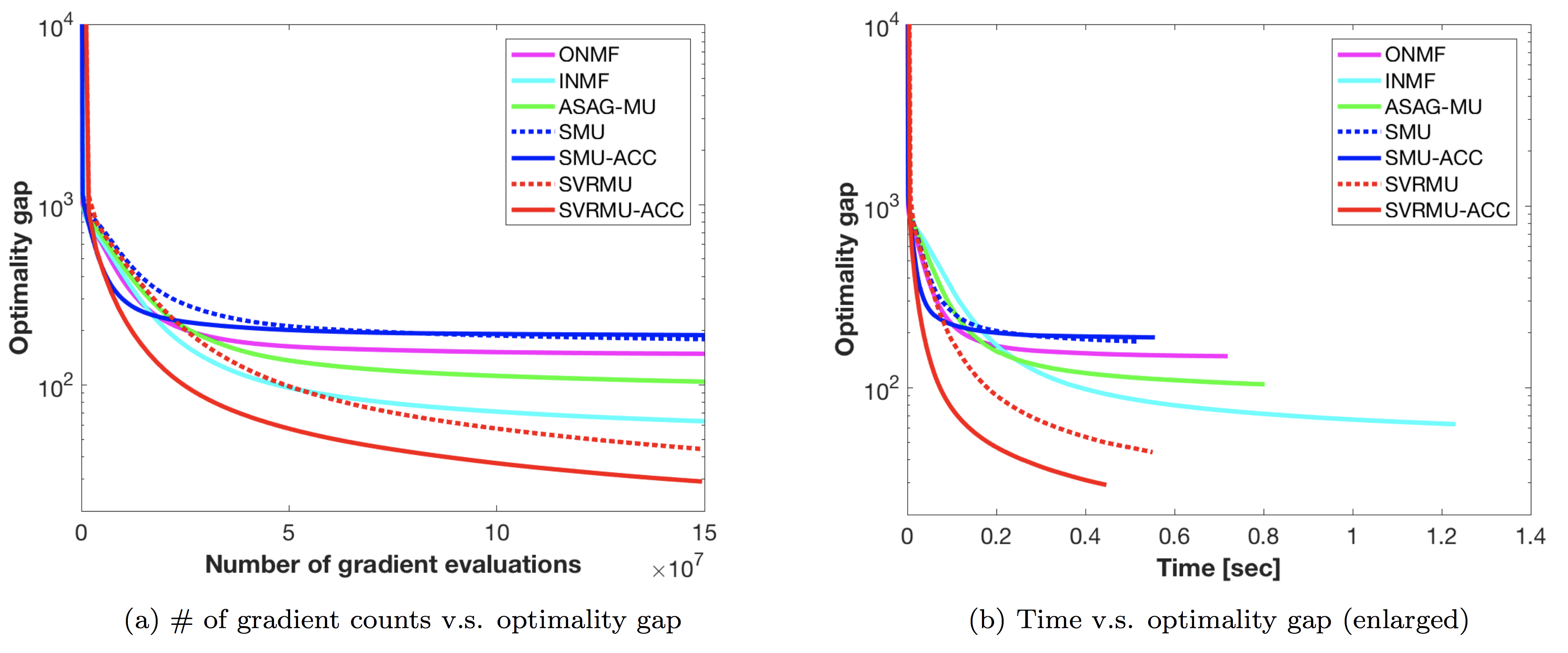
Nonnegative matrix factorization (NMF), a matrix decomposition, a dimensionality reduction and factor analysis method, is a special case in which factor matrices have low-rank nonnegative constraints. Considering the stochastic learning in NMF, we specifically address the multiplicative update (MU) rule, which is the most popular, but which has slow convergence property. This code provides a solver of the stochastic MU rule with a variance-reduced (VR) technique of stochastic gradient, called SVRMU. Numerical comparisons suggest that SVRMU robustly outperforms state-of-the-art algorithms across different synthetic and real-world datasets.
| Algorithm name in example codes | function | options |
|---|---|---|
| SMU | smu_nmf |
|
| SMU-ACC | smu_nmf |
accel=1&rep_mode = 'fix' |
| SMU-ACC-Adaptive | smu_nmf |
accel=1&rep_mode = 'adaptive' |
| SMU-LS | smu_nmf |
ls=1 |
| SMU-LS-ACC | smu_nmf |
accel=1&ls=1 |
| SVRMU | svrmu_nmf |
|
| SVRMU-ACC | svrmu_nmf |
accel=1&rep_mode = 'fix' |
| SVRMU-ACC-Adaptive | svrmu_nmf |
accel=1&rep_mode = 'adaptive' |
| SVRMU-LS | svrmu_nmf |
ls=1 |
| SVRMU-LS-ACC | svrmu_nmf |
accel=1&ls=1 |
| SVRMU-Precon-LS | svrmu_nmf |
ls=1&precon = 1 |
| SVRMU-Precon-LS-ACC | svrmu_nmf |
accel=1&ls=1&precon = 1 |
| RSVRMU | svrmu_nmf |
robust=true |
| RSVRMU-ACC | svrmu_nmf |
robust=true&accel=1&rep_mode = 'fix' |
| RSVRMU-LS | svrmu_nmf |
robust=true&ls=1 |
- SVRMU-ACC-XXX
- Accelerated variant of SVRMU
- RSVRMU-XXX
- Robust variant of SVRMU
./                                      - Top directory of NMFLibrary.
./test_nmf_online.m                     - Demo file for SMU and SVRMU algorithms.
./solver/online/svrmu_nmf.m             - SVRMU algorithm file.
./solver/online/smu_nmf.m               - SMU algorithm file.
./test/comp_nmf_online_algorithms       - Comparison file for solvers.
./test/demo_face_online.m               - Demo file for face datasets.
./test/demo_face_with_outlier_online.m  - Demo file for face datasets with outlier.
Obtain the NMFLibrary package. Then, follow below.
%% First run the setup script
run_me_first; Just execute test_nmf_online for a simplest demonstration of the SVRMU algorithm.
%% Execute the demonstration script
demo; "test_nmf_online.m" file contains below.
%% generate synthetic data non-negative matrix V size of (FxN)
F = 300;
N = 1000;
V = rand(F,N);

%% Initialize rank to be factorized
K = 5;

%% Set batchsize
options.batch_size = N/10;

%% perform factroization
% SMU
[w_smu_nmf, infos_smu_nmf] = smu_nmf(V, K, options);
% SVRMU
[w_svrmu_nmf, infos_svrmu_nmf] = svrmu_nmf(V, K, options);

%% plot
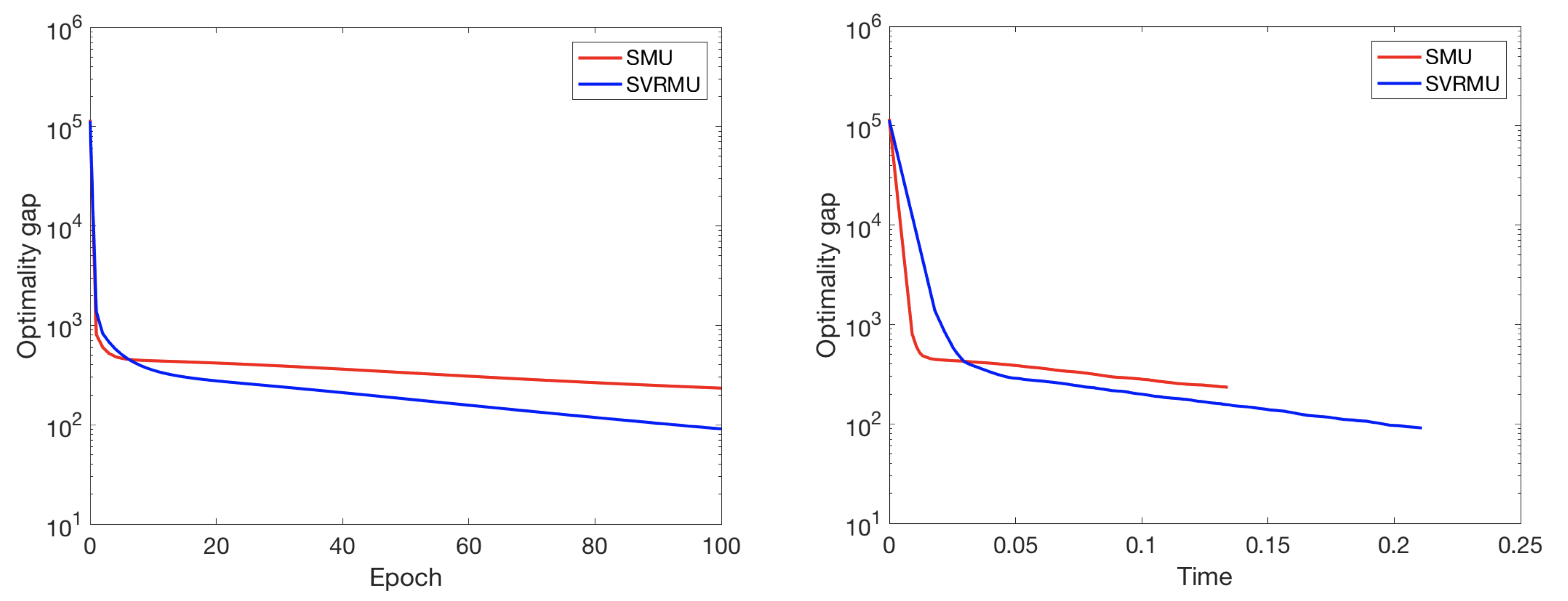
display_graph('epoch','cost', {'SMU', 'SVRMU'}, {w_smu_nmf, w_svrmu_nmf}, {infos_smu_nmf, infos_svrmu_nmf});
display_graph('time','cost', {'SMU', 'SVRMU'}, {w_smu_nmf, w_svrmu_nmf}, {infos_smu_nmf, infos_svrmu_nmf});
Let's take a closer look at the code above bit by bit. The procedure has only 4 steps!
Step 1: Generate data
First, we generate synthetic data of V of size (FxN).
F = 300;
N = 1000;
V = rand(F,N);
Step 2: Define rank
We set the rank value.
K = 5;Step 3: Perform solver
Now, you can perform optimization solvers, e.g., SMU and SVRMU, calling solver functions, i.e., smu_nmf() function and svrmu_nmf() function after setting some optimization options.
options.batch_size = N/10;

% SMU
[w_smu_nmf, infos_smu_nmf] = smu_nmf(V, K, options);
% SVRMU
[w_svrmu_nmf, infos_svrmu_nmf] = svrmu_nmf(V, K, options);
They return the final solutions of w and the statistics information that include the histories of epoch numbers, cost values, norms of gradient, the number of gradient evaluations and so on.
Step 4: Show result
Finally, display_graph() provides output results of decreasing behavior of the cost values in terms of the number of iterrations (epochs) and time [sec].
display_graph('epoch','cost', {'SMU', 'SVRMU'}, {w_smu_nmf, w_svrmu_nmf}, {infos_smu_nmf, infos_svrmu_nmf});
display_graph('time','cost', {'SMU', 'SVRMU'}, {w_smu_nmf, w_svrmu_nmf}, {infos_smu_nmf, infos_svrmu_nmf});
That's it!
- Demonstation using face datasets
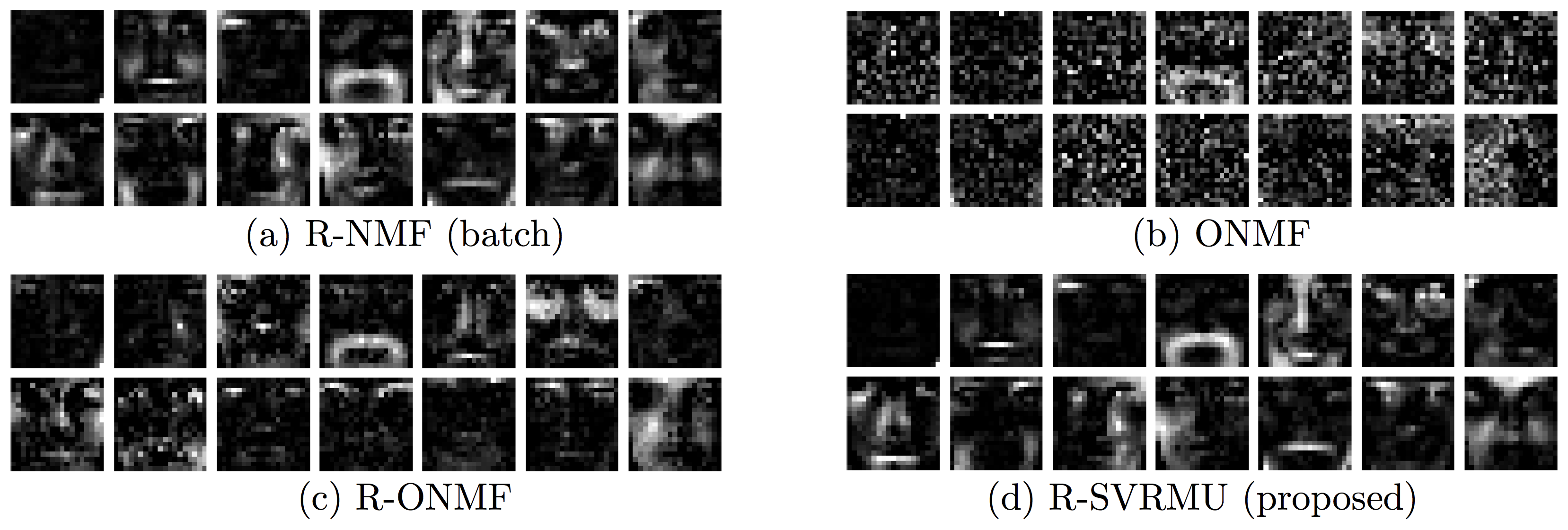
"demo_face_online.m" in the "test" folder illustrates the learned basis (dictrionary). THis demo uses CBCL face datasets datasets.
The dataset is first loaded into V instead of generating synthetic data in Step 1.
V = importdata('../data/CBCL_Face.mat');
V = V(:,1:N); % get partial matrix
V = normalization(V, 50); % set max_level=50
Then, we can display basis elements (W: dictionary) obtained with different algorithms additionally in Step 4.
plot_dictionnary(w_smu_nmf.W, [], [7 7]);
plot_dictionnary(w_svrmu_nmf.W, [], [7 7]); - Demonstation of robust variant
"demo_face_with_outlier_online.m" in the "test" folder illustrates the learned basis of face datasets with outlier.
After loading the dataset, outlier is added in Step 1.
% set outlier level
outlier_rho = 0.2;
% add outliers
[V, ~] = add_outlier(outlier_rho, F, N, V);
Then, you can call the robust mode by setting options.robust=true in Step 3.
options.robust = true;
[w_svrmu_nmf, infos_svrmu_nmf] = svrmu_nmf(V, K, options); - The code is free, non-commercial and open source.
- The code provided should only be used for academic/research purposes.
If you have any problems or questions, please contact the author: Hiroyuki Kasai (email: kasai at is dot uec dot ac dot jp)
- Version 1.0.0 (Apr. 17, 2018)
- Initial version.


